Chapter 1: Discrete Geometric Quantities and Operators

import igl
import scipy as sp
import numpy as np
from meshplot import plot, subplot, interact

import os
root_folder = os.getcwd()
#root_folder = os.path.join(os.getcwd(), "tutorial")

This chapter illustrates a few discrete quantities that libigl can compute on a mesh and the libigl functions that construct popular discrete differential geometry operators. It also provides an introduction to basic drawing and coloring routines of our viewer.

Gaussian curvature

Gaussian curvature on a continuous surface is defined as the product of the principal curvatures:

$k_G = k_1 k_2.$

As an intrinsic measure, it depends on the metric and not the surface’s embedding.

Intuitively, Gaussian curvature tells how locally spherical or elliptic the surface is ( $k_G>0$ ), how locally saddle-shaped or hyperbolic the surface is ( $k_G<0$ ), or how locally cylindrical or parabolic ( $k_G=0$ ) the surface is.

In the discrete setting, one definition for a “discrete Gaussian curvature” on a triangle mesh is via a vertex’s angular deficit:

$k_G(v_i) = 2π - \sum\limits_{j\in N(i)}θ_{ij},$

where $N(i)$ are the triangles incident on vertex $i$ and $θ_{ij}$ is the angle at vertex $i$ in triangle $j$ (Meyer, 2003).

Just like the continuous analog, our discrete Gaussian curvature reveals elliptic, hyperbolic and parabolic vertices on the domain.

Let’s compute Gaussian curvature and visualize it in pseudocolor. First, calculate the curvature with libigl and then plot it in pseudocolors.

v, f = igl.read_triangle_mesh(os.path.join(root_folder, "data", "bumpy.off"))
k = igl.gaussian_curvature(v, f)
plot(v, f, k)

Next, compute the massmatrix and divide the gaussian curvature values by area to get the integral average.

m = igl.massmatrix(v, f, igl.MASSMATRIX_TYPE_VORONOI)
minv = sp.sparse.diags(1 / m.diagonal())
kn = minv.dot(k)
plot(v, f, kn)

Curvature directions

The two principal curvatures $(k_1,k_2)$ at a point on a surface measure how much the surface bends in different directions. The directions of maximum and minimum (signed) bending are called principal directions and are always orthogonal.

Mean curvature is defined as the average of principal curvatures:

$H = \frac{1}{2}(k_1 + k_2).$

One way to extract mean curvature is by examining the Laplace-Beltrami operator applied to the surface positions. The result is a so-called mean-curvature normal:

$-\Delta \mathbf{x} = H \mathbf{n}.$

It is easy to compute this on a discrete triangle mesh in libigl using the cotangent Laplace-Beltrami operator (Meyer, 2003).

l = igl.cotmatrix(v, f)
m = igl.massmatrix(v, f, igl.MASSMATRIX_TYPE_VORONOI)

minv = sp.sparse.diags(1 / m.diagonal())

hn = -minv.dot(l.dot(v))
h = np.linalg.norm(hn, axis=1)
plot(v, f, h)

Combined with the angle defect definition of discrete Gaussian curvature, one can define principal curvatures and use least squares fitting to find directions (Meyer, 2003).

Alternatively, a robust method for determining principal curvatures is via quadric fitting (Panozzo, 2010). In the neighborhood around every vertex, a best-fit quadric is found and principal curvature values and directions are analytically computed on this quadric.

v1, v2, k1, k2 = igl.principal_curvature(v, f)
h2 = 0.5 * (k1 + k2)
p = plot(v, f, h2, shading={"wireframe": False}, return_plot=True)

avg = igl.avg_edge_length(v, f) / 2.0
p.add_lines(v + v1 * avg, v - v1 * avg, shading={"line_color": "red"})
p.add_lines(v + v2 * avg, v - v2 * avg, shading={"line_color": "green"})

Gradient

Scalar functions on a surface can be discretized as a piecewise linear function with values defined at each mesh vertex:

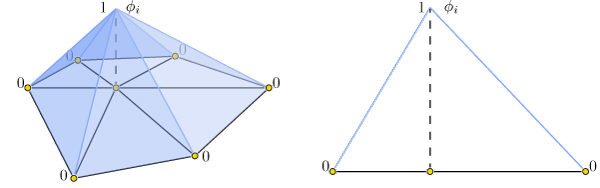
$f(\mathbf{x}) \approx \sum\limits_{i=1}^n \phi_i(\mathbf{x})\, f_i,$

where $\phi_i$ is a piecewise linear hat function defined by the mesh so that for each triangle $\phi_i$ is the linear function which is one only at vertex $i$ and zero at the other corners.

Thus gradients of such piecewise linear functions are simply sums of gradients of the hat functions:

$\nabla f(\mathbf{x}) \approx \nabla \sum\limits_{i=1}^n \phi_i(\mathbf{x})\, f_i = \sum\limits_{i=1}^n \nabla \phi_i(\mathbf{x})\, f_i.$

This reveals that the gradient is a linear function of the vector of $f_i$ values. Because the $\phi_i$ are linear in each triangle, their gradients are constant in each triangle. Thus our discrete gradient operator can be written as a matrix multiplication taking vertex values to triangle values:

$\nabla f \approx \mathbf{G}\,\mathbf{f},$

where $\mathbf{f}$ is $n\times 1$ and $\mathbf{G}$ is an $md\times n$ sparse matrix. This matrix $\mathbf{G}$ can be derived geometrically (Jacobson, 2013).

Libigl’s grad function computes $\mathbf{G}$ for triangle and tetrahedral meshes. Let’s see how this works. First load a mesh and a corresponding surface function. Next, compute the gradient operator g (#F*3 x #V) on the triangle mesh, apply it to the surface function and extract the magnitude.

v, f = igl.read_triangle_mesh(os.path.join(root_folder, "data", "cheburashka.off"))
u = igl.read_dmat(os.path.join(root_folder, "data", "cheburashka-scalar.dmat"))

g = igl.grad(v, f)
gu = g.dot(u).reshape(f.shape, order="F")

gu_mag = np.linalg.norm(gu, axis=1)
p = plot(v, f, u, shading={"wireframe":False}, return_plot=True)

max_size = igl.avg_edge_length(v, f) / np.mean(gu_mag)
bc = igl.barycenter(v, f)
bcn = bc + max_size * gu
p.add_lines(bc, bcn, shading={"line_color": "black"})